Filmic Tonemapping Curve

Tonemapping is used to achieve visually-pleasing rendering of high dynamic range scenes, e.g. those captured by HDR cameras or simulated by computer graphics. It is commonly attained by applying an S-shaped curve to the intensity channel. The curve is called “filmic” by analogy with the characteristic curve of a typical photosensitive material.

Four parameters are commonly used to define the shape of the curve: toe length, toe strength, shoulder length and shoulder strength. A popular approach for consructing the curve based on power functions was described by John Hable. It produces excellent results but the conversion from the four parameters given above to those used in calculations is somewhat complex and indirect. This post describes an alternative approach.

Bézier curves

French engineer Pierre Bézier (1910–1999) came up with a brilliant way to define a smoothing curve. He used it for designing the bodywork of Renault cars in the 1960s. Bézier curves became widely adopted in computer graphics, robotics and other domains.

Given three points \(P_0\), \(P_1\) and \(P_2\) the quadratic Bézier curve is defined as follows:

$$B(t)=(1-t)^{2}{P}_{0}+2(1-t){P}_{1}+t^{2}{P}_{2}$$

where \(0\leq t\leq 1\) is a parameter.

Application

Adapting Bézier curves for tone mapping is a faily straightforward task. The linear part of the tone curve (between the toe and the shoulder) is described by the following equation:

$$y(x)=\frac{t_{S} + s_{S} - 1}{t_{L} + s_{L} - 1}(x - t_{L}) + t_{S}$$

where \(t_{L}\), \(t_{S}\), \(s_{L}\) and \(s_{S}\) are toe length, toe strength, shoulder length and shoulder strength, respectively; \(x\) is the input tone normalized to the \([0, 1]\) range, and \(y\) is the tone-mapped output.

Consider the shoulder part of the curve first. The three points defining the curve are:

$$ \begin{flalign*} &\quad P_{0}=(1-s_{L}, 1-s_{S}) & \\ &\quad P_{1}=((1 - t_{S})\frac{t_{L} + s_{L} - 1}{t_{S} + s_{S} - 1} + t_{L}, 1) & \\ &\quad P_{2}=(1, 1) & \\ \end{flalign*} $$

Substituting these in the equation for \(B(t)\) will give two parametric equations for \(x(t)\) and \(y(t)\). We can now solve a quadratic equation for the parameter \(t_{1}\) and get the following expressions:

$$ y(x)=(1 - t_{1})^{2}(1 - s_{S}) + 2(1 - t_{1})t_{1} + {t_{1}}^2 $$

where

$$ \begin{flalign*} &\quad t_{1}=\frac{-(x_{1} + s_{L} - 1) + \sqrt{({x_{1} + s_{L} - 1})^2 - (2 - 2x_{1} - s_{L})(1 - s_{L} - x)}}{2 - 2x_{1} - s_{L}} & \\ &\quad x_{1}=(1 - t_{S})\frac{t_{L} + s_{L} - 1}{t_{S} + s_{S} - 1} + t_{L} & \\ \end{flalign*} $$

The toe part of the curve is derived similarly.

The Final Curve

The resulting tone mapping curve \(y(x)\) is:

$$y(x)=\left\{ \begin{array}{ l l } 0 & \textrm{if } x \leq 0 \\ {{t_{0}}^2}t_{S} & \textrm{if } 0 < x \leq t_{L} \\ \frac{t_{S} + s_{S} - 1}{t_{L} + s_{L} - 1}(x - t_{L}) + t_{S} & \textrm{if } t_{L} < x \leq 1-s_{L} \\ (1 - t_{1})^{2}(1 - s_{S}) + 2(1 - t_{1})t_{1} + {t_{1}}^2 & \textrm{if } 1 - s_{L} < x \leq 1 \\ 1 & \textrm{otherwise } \end{array} \right.$$

where

$$ \begin{flalign*} &\quad t_{0} = \frac{-x_{0} + \sqrt{{x_{0}}^2 + (t_{L} - 2x_{0})x}} {t_{L} - 2x_{0}} & \\ &\quad x_{0} = -t_{S}\frac{t_{L} + s_{L} - 1} {t_{S} + s_{S} - 1} + t_{L} & \\ \end{flalign*} $$

Example

To demonstrate the application of the tonemapping curve a RAW image captured by a digital camera was imported using XYZ color space and linear gamma. The original and the tone mapped images are shown below (move the slider to see the change).

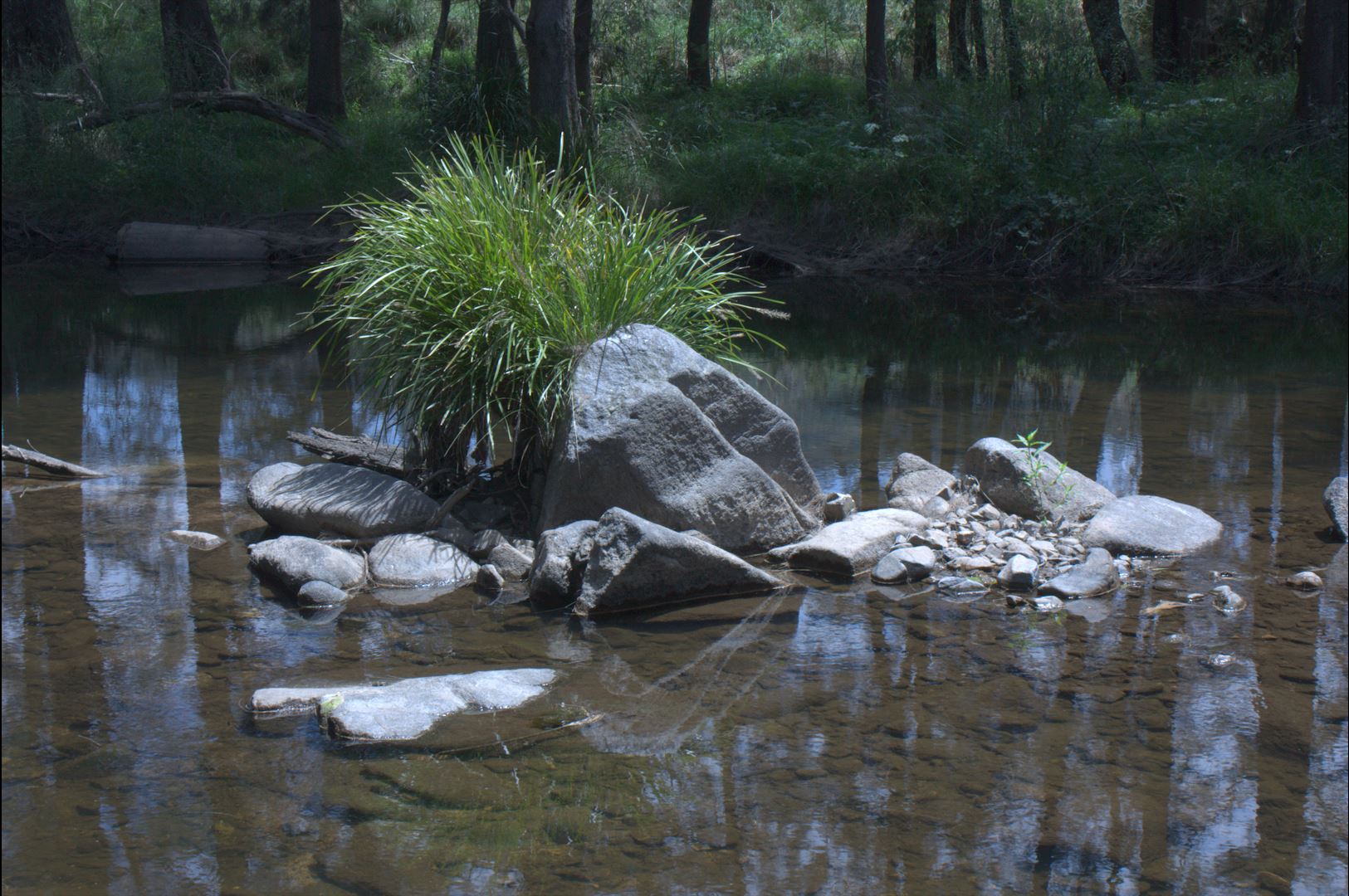
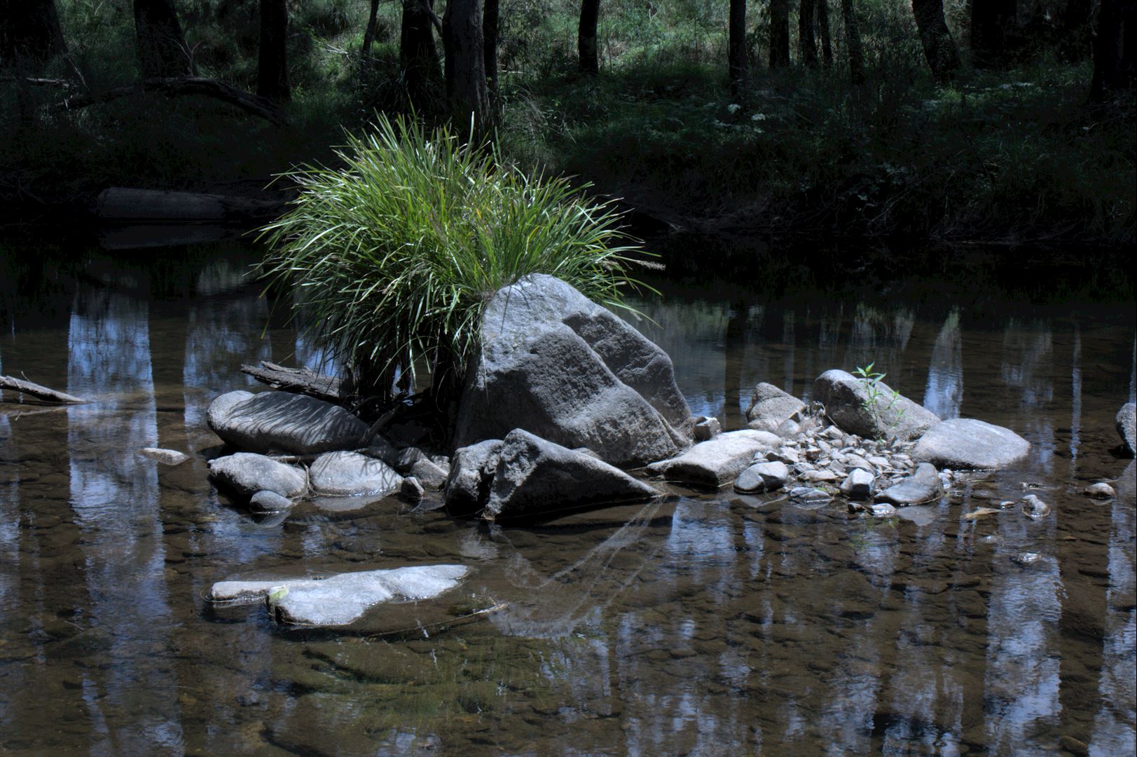
The tone curve had the following parameters: \(t_{L}=0.05\), \(t_{S}=0.025\), \(s_{L}=0.26\) and \(s_{S}=0.3\).

Implementation

Direct implementation of the tone mapping based on Bézier curves is expected to be slower than the power function curve proposed by John Hable. A more efficient implementation could use a look-up table (LUT) for the toe and shoulder and direct calculation for the linear part of the curve. For most images the majority of pixels would fall on the linear part and the overall effect on the performance is expected be small.

Tone mapping is best applied in the XYZ color space. The scaling factor could be calculated using the values of the Y channel, and then applied to all three channels. This way the color values of the image will be preserved. The resulting tonemapped image must be normalized to avoid clipping the highlights.

Conclusion

An alternative approach for defining tone mapping curves is proposed that uses Bézier curves and direct parametes of the length and strength of the toe and the shoulder region. With careful implementation its performance is expected to be on par with the widely used power function curve method.